Noise is the indispensable part of the information today such that it may corrupt the information either partly or fully. In images, noises can obscure a part of the image or may corrupt the image in a way to spoil all of it. Salt & Pepper is a kind of noise that is generally caused by the sudden signal disturbances in the image signal.
In order to clean out the images from the noises, filters are applied. Especially for the Salt & Pepper noise, a median filter is applied generally. Below median filter is explained with an example then different strategies of median filter are introduced, python implementations are also given with an example.
Median Filter
Generally, filters are applied with a small, usually square, window or kernel sliding on the noisy image. For example, a kernel of size 3x3 is given below.
5 7 15 0 9 4 21 6 1
Generally center of the kernel is the (1, 1) location, in this example its intensity is 9. So, in order to apply the median filter, first the kernel must be row wise expanded and then sorted.
Row wise expand :
5 7 15 0 9 4 21 6 1
Sort :
0 1 4 5 6 7 9 15 21]
Now the median of the sorted array is the value to pick and put on the noisy image at the center of the kernel. So after applying the filter, the median value which is 6 is picked and replaced with the 9 in the location of the center of the kernel.
For gray scale images, since they are single channel, only checking the intensity value is enough but for color images, since there are generally 3 channels (r, g, b) a method is needed to apply the median filter.
Median Filter Strategies for Color Images
As stated above, color images are made up of 3 channels aka red, green and blue channels. In order to clean out the Salt & Pepper noise in color images, there are different strategies to apply.
The strategies can be divided into two groups being either marginal or scalar ordering. The marginal ordering strategy behaves to the channels separately, i.e applies the median filters to the channels separately, considering no relations between the channels. On the other hand, scalar ordering strategy behaves to the channels as a one unit, applies the filters by considering the channels together.
So there are different methods for color images because of the ordering problem. For binary and gray scale images, the ordering is easily satisfied using either “<=” or “>=” mathematical operators for the intensities. For example, as shown above, a frame can be ordered by comparing the intensity values with “<=” operator. To be more precise, consider the (0, 0) and (0, 1) pixels whose intensity values are 5 and 7 respectively. The operator “<=” can be used between these values to decide to the result of the comparison. But for a color image, there are three channels, it is not as easy to decide which pixel is smaller or bigger.
Consider these three RGB pixels for the strategies explained below :
1st pixel – 5 15 0 2nd pixel – 1 8 5 3rd pixel – 1 9 4
Marginal Median Filtering Strategy
Marginal strategy, as stated above, behaves to the channels independently. So it separates the channels and orders the corresponding intensities. For example :
First channel is ordered like: 1 1 5
Second channel is ordered like: 8 9 15
Third channel is ordered like: 0 4 5
The median values of these independent ordered lists are selected [1, 9, 4] as the new color pixel to replace. Below written a simple python implementation for this strategy in order to give the intuition, which is also shared as a gist.
def medianFilterMarginal(img, filterSize = 3):
    imgHeight, imWidth, channels = img.shape
    outputImg = np.zeros((imgHeight, imWidth, channels),dtype=np.uint8)

    filterHeight = filterWidth = filterSize
    filterEdge = filterWidth // 2

    for i in range(filterEdge,imgHeight - filterEdge):
        for j in range(filterEdge,imWidth - filterEdge):
            # get a frame around the pixel by the filter size
            imgFilter = img[i - filterEdge : i + filterEdge + 1, j - filterEdge : j + filterEdge + 1]

            # seperate channels, reshape to a one dimensional array and sort it
            red = np.sort(imgFilter[:, :, 0].reshape(filterHeight * filterWidth))
            green = np.sort(imgFilter[:, :, 1].reshape(filterHeight * filterWidth))
            blue = np.sort(imgFilter[:, :, 2].reshape(filterHeight * filterWidth))

            # get the median intensity
            outputImg[i][j][0] = red[(filterWidth * filterHeight) // 2]
            outputImg[i][j][1] = green[(filterWidth * filterHeight) // 2]
            outputImg[i][j][2] = blue[(filterWidth * filterHeight) // 2]

    return outputImg
Scalar Median Filtering Strategy
Scalar strategy, as stated above, behaves to the channels as a one unit. There are different scalar strategies using different ordering methods. One of the methods uses a lexical ordering, like looking out a word from a dictionary.
Lexical Ordering
With lexical ordering, intensity values of the corresponding channels between the pixels are compared and the pixels are ordered according to their place in lexical order. For the example pixels given above, pixels are lexically ordered like : [ [1, 8, 5], [1, 9, 4], [5, 15, 0] ]. Then the median of the list which is [1, 9, 4] is picked to replace. As seen, the pixels with 3 channels are treated as a one unit, instead of doing separate calculations like in marginal ordering.
Below given a simple python implementation for this ordering strategy with gist.
def medianFilterLexicalOrdering(img, filterSize = 3):
    imgHeight, imWidth, channels = img.shape
    outputImg = np.zeros((imgHeight, imWidth, channels), dtype=np.uint8)

    filterHeight = filterWidth = filterSize
    filterEdge = filterWidth // 2

    for i in range(filterEdge, imgHeight - filterEdge):
        for j in range(filterEdge, imWidth - filterEdge):
            # retrieve a frame around the pixel i,j to check
            imgFilter = img[i - filterEdge : i + filterEdge + 1, j - filterEdge : j + filterEdge + 1].reshape(filterHeight * filterWidth, channels)

            # rotate the frame, lexically sort and get the indices of the order
            lexSortedIndexes = np.lexsort(np.rot90(imgFilter))

            # get the median index of the lexically sorted values, put its intensity
            outputImg[i][j] = imgFilter[lexSortedIndexes[(filterWidth * filterHeight // 2)]]

    return outputImg
Norm Based Ordering
With norm based ordering, pixels are ordered with respect to the norm of the channels, thinking it like a vector of size 3. For the example given above, first norm of the pixels are calculated.
Norm of the [5, 15, 0] is 15.8.
Norm of the [1, 8, 5] is 9.5.
Norm of the [1, 9, 4] is 9.9.
So the pixels are ordered with respect to their norms :
1 8 5 1 9 4 5 15 0
Then the median of the list is which is [1, 9, 4] picked to replace. Below given a simple python implementation for this ordering strategy with gist.
def medianFilterLexicalOrdering(img, filterSize = 3):
    imgHeight, imWidth, channels = img.shape
    outputImg = np.zeros((imgHeight, imWidth, channels), dtype=np.uint8)

    filterHeight = filterWidth = filterSize
    filterEdge = filterWidth // 2

    for i in range(filterEdge, imgHeight - filterEdge):
        for j in range(filterEdge, imWidth - filterEdge):
            # retrieve a frame around the pixel i,j to check
            imgFilter = img[i - filterEdge : i + filterEdge + 1, j - filterEdge : j + filterEdge + 1].reshape(filterHeight * filterWidth, channels)

            # rotate the frame, lexically sort and get the indices of the order
            lexSortedIndexes = np.lexsort(np.rot90(imgFilter))

            # get the median index of the lexically sorted values, put its intensity
            outputImg[i][j] = imgFilter[lexSortedIndexes[(filterWidth * filterHeight // 2)]]

    return outputImg
Results
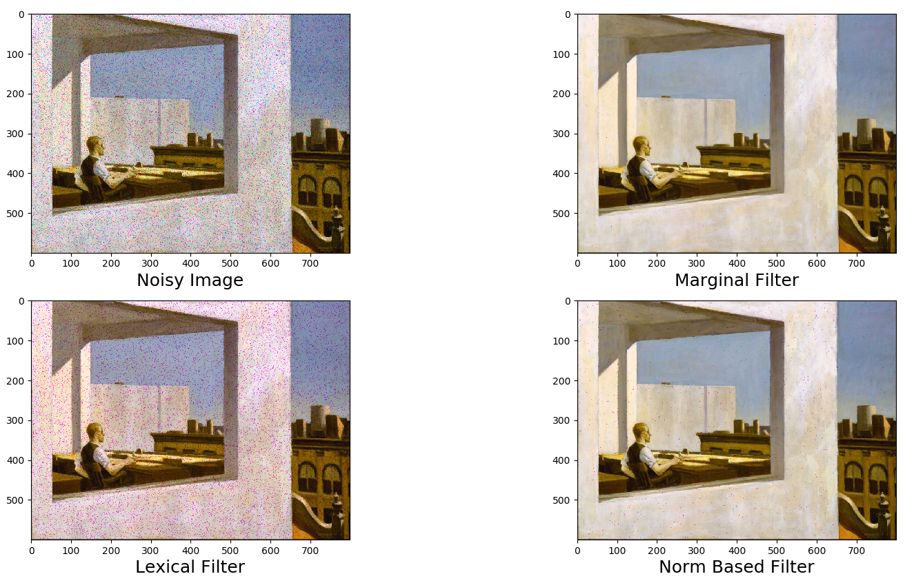
Here these different median filter strategies are applied to a noisy image to compare their performance. In order to give the basic intuition these filters are applied to a single image, but under different circumstances performance of these filters may vary. After experiments on different images, with different filter sizes and noise amount, observed things :
- Generally marginal strategy achieves better than the others and the scalar methods perform similar where lexicographical ordering performs worse than others generally.
- Marginal strategy at various noise levels achieves better performance, scalar methods perform similar.
- Norm-based ordering is not affected much by the filter size unlike others but still marginal strategy achieves better performance.
- There is a case where norm-based ordering beats all others which is a high level of noise with bigger filter size.
- Padding of the filter, affects the performance significantly. Using zero padding instead of filling with original pixels performs better.
Below an example image from Edward Hopper is given with a Salt & Pepper noise at 0.05 ratio. Then three different strategies explained above are applied to filter out the noise. As stated in above observations, marginal filter almost cleans out all the noise, while lexical ordering filter performs the worst and norm based filters better than the lexical ordering.