
This post compiles notes from the notebook I prepared for a recitation I conducted in Sabanci University when I was a teaching assistant of the machine learning course.
What is Dimensionality Reduction?
Wikipedia: Dimensionality reduction is the transformation of data from a high-dimensional space into a low-dimensional space so that the low-dimensional representation retains some meaningful properties of the original data.
Useful technique to:
- Eliminiate unrelated, unsupportive features and select more suitable features
- Extract new features from the existing ones
- Help reduce a noise
- Ease data visualization for better EDA
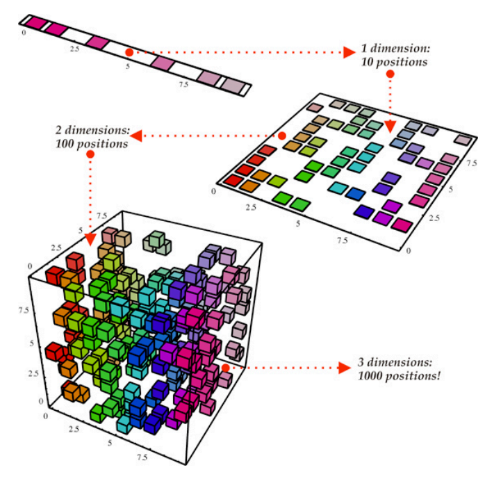
- Prevent from curse of dimensionality
- Wikipedia: When the dimensionality increases, the volume of the space increases so fast that the available data become sparse. In order to obtain a reliable result, the amount of data needed often grows exponentially with the dimensionality.
Information loss?
- The techniques try to retain as much of the information as possible while reducing the dimension/selecting related features.
Two types of transformation:
1- Linear: linear projection of data onto a lower dimensional space
1- Principal Component Analysis (PCA)
2- Linear Discriminany Analysis (LDA)
3- Factor Analysis
2- Non Linear: non linear projection of data onto a lower dimensional space
1- Kernel based PCA
2- t-distributed Stochastic Neighbor Embedding (t-SNE)
3. Auto-Encoder
Principal Component Analysis
Wikipedia: The process of computing the principal components and using them to perform a change of basis on the data, sometimes using only the first few principal components and ignoring the rest.
Can be summarized in four steps:
1. Standardize the data to the same scale
- Center and scale the data
- To prevent from bigger scales dominating lower ones (0-100 vs 0-1)
- e.g. Height (cm) vs Weight (kg)
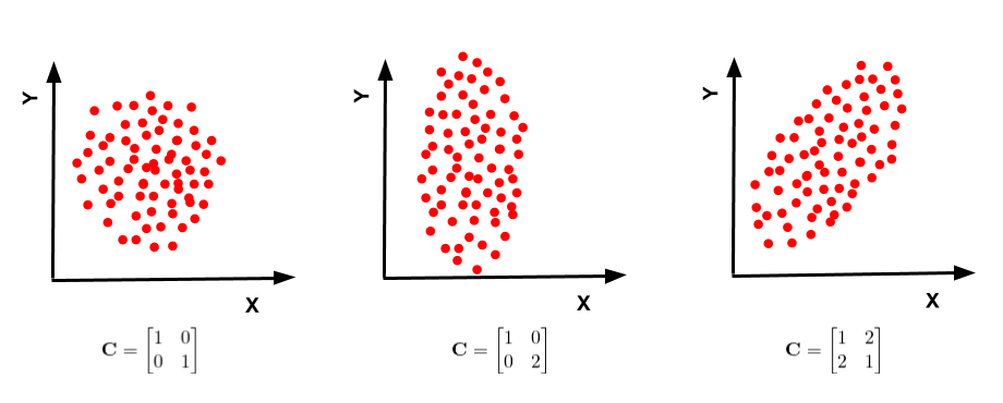
2. Compute the covariance matrix
- To identify relationship between the original data and the mean of the data
- i.e How the data varies from the mean
3. Compute the eigenvectors and eigenvalues to find principal components
    - Principal component shows the direction of data having maximum variance
    - Variance: the average of the squared distances from the projected points (red dots) to the origin (from the same link of the gif)
- Eigenvectors of the Covariance matrix are actually the directions of the axes where there is the most variance(most information) and that we call Principal Components.
- Eigenvalues are simply the coefficients attached to eigenvectors, which give the amount of variance carried in each Principal Component. (from the same link of the gif)
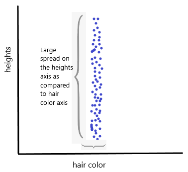
- Why do we consider variance?
    - Almost, all people have similar hair color.
    - Yet, height varies much more, which makes it more important.
4. Select k number of principal components as the project data
    - Sort the principal components wrt. eigenvalues
    - Select k number of components according to your needs
5. Organize the selected principal components as new axis
Geometrically, we rotate our axes after doing standardization. Since there are d dimensions so we’ll get d eigen vectors and d eigen values. For each eigen vector we project points on the vector and measure the variance or spread i.e. eigen value and in the end the vector with highest eigen values our principal component. Now that we have new dimensions or features the values of these features are the projection of points on these vectors. Now if we like we can decide to ignore the components of lesser significance. We do loose some information, but if the eigen values are small, we don’t loose much. If we leave out some components, the final dataset will have less dimensions than the original.
from https://medium.com/@ashwin8april/dimensionality-reduction-and-visualization-using-pca-principal-component-analysis-8489b46c2ae0
- How to explain PCA to a layman? Answer: https://stats.stackexchange.com/questions/2691/making-sense-of-principal-component-analysis-eigenvectors-eigenvalues.
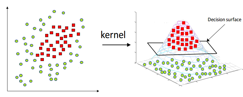
Kernel Based PCA
While PCA can capture the data on linear manifold, it fails for non-linear cases.
Kernel PCA first projects the data onto a higher dimensional space to make it linearly separable then follows similar steps to PCA.
With Kernel PCA:
1- A kernel function is choosen (e.g. Gaussian)
2- Compute the kernel matrix, similar to covariance matrix in PCA
3- Center the kernel matrix

- From now on, similar to PCA:

4- Compute the eigenvectors and values
5- Select k number of principal components
6- Organize the selected components as new axis
Take a look at this link for a good explanation of advantageous of the Kernel PCA over PCA.
t - SNE
Wikipedia: Well-suited for embedding high-dimensional data for visualization in a low-dimensional space.
Models each high-dimensional object by a two- or three-dimensional point in such a way that similar objects are modeled by nearby points and dissimilar objects are modeled by distant points with high probability.
Sklearn: Converts similarities between data points to joint probabilities and tries to minimize the Kullback-Leibler divergence between the joint probabilities of the low-dimensional embedding and the high-dimensional data.
- Constructs a probability distribution over pairs of high-dimensional objects in such a way that similar objects are assigned a higher probability while dissimilar points are assigned a lower probability.
- Defines a similar probability distribution over the points in the low-dimensional map, and it minimizes the Kullback–Leibler divergence (KL divergence) between the two distributions with respect to the locations of the points in the map.
Please take a look at this link of Laurens van der Maaten for more examples, FAQ and different programming languages based implementations.
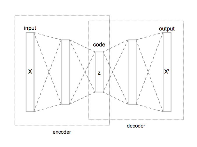
Auto - Encoder
It is an unsupervised, artificial neural network consisting of encoder & decoder modules.
-
Encoder projects the input data to a lower dimension than the input data dimension i.e. compresses (encodes) the information.
-
Decoder reconstructs the compressed (encoded) representation to the original input data.
-
The parameters of the model is usually optimized with respect to mean squared error.
-
The dimensionality reduced version of the input data resides in the encoded represenatation.
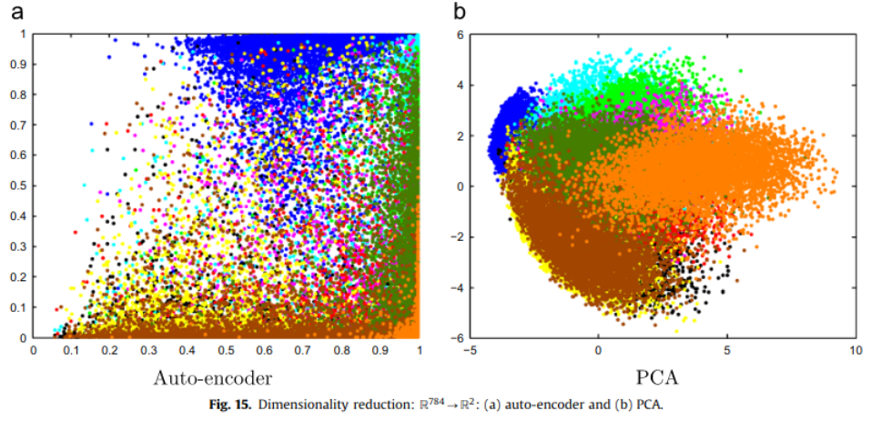
- Comparison with PCA:
| Auto Encoder | PCA |
|---|---|
| Non linear. | Linear. |
| Trained wrt. gradient descent, too long. | Pretty fast. |
| Better for more complex data | Better for simpler data |
ps:
-
Typically, linear algebra and manifold learning methods assume that all input features have the same scale or distribution. This suggests that it is good practice to either normalize or standardize data prior to using these methods if the input variables have differing scales or units.
-
Any dimensionality reduction performed on training data must also be performed on new data, such as a test dataset, validation dataset, and data when making a prediction with the final model.